Project summary
This project demonstrates a complete, production-style data and machine learning workflow, built from scratch using modern engineering and MLOps practices. The solution simulates realistic sales data, processes it through a data engineering pipeline, trains ML models to forecast product demand, and deploys the model as a fully containerized API with automated CI/CD.
Business context
Inventory forecasting is a common challenge in retail operations. A fictional retail company, MarketFlow, wants to improve its inventory management. Every day, thousands of sales are registered across different regions, but the company struggles to anticipate how much of each product will be sold. This results in overstock in some cities and product shortages in others, increasing storage costs and reducing customer satisfaction.
In addition, the company currently has limited analytical capabilities and lacks a structured process to analyze historical sales data. Because of this, decision-making is often reactive rather than data-driven. MarketFlow wants to develop a solid analytical foundation—starting with dashboards, KPIs, and exploratory analysis—and then build sales forecasting models to support smarter inventory planning and operational efficiency.
Objectives
- Build a data-driven system that predicts the sales quantity.
With this objective the business will be able to optimize inventory levels, plan logistics more efficiently, and reduce costs by avoiding lost sales.
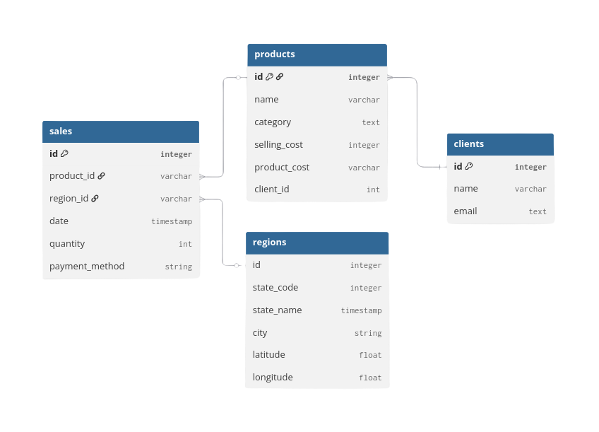
Database schema
The dataset consists of four main tables—sales, products, regions, and clients. In this project we focus on the sales and regions tables.
Further links
Data acquisition
For this project, the data was collected using a fake-data generator API. This tool helped gather simulated data across different date ranges and for varying numbers of clients. It generates realistic data that follows customizable patterns, making it a great resource for personal projects and learning.
Currently, the project hasn't been released to the public due to some technical details that I still need to fix in the API. If you want further information, please feel free to email me.
Data collection, storage and processing
Once the initial parameters for data simulation are established (e.g., number of clients, number of stores, amount of injected errors), the tool allows you to generate data incrementally up to the current day.
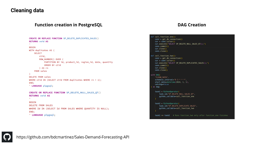
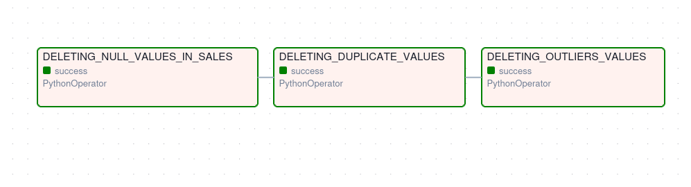
Based on this process, an Airflow DAG was created to retrieve the data each day and store it in a PostgreSQL database. The data is then cleaned using predefined functions (similar to stored procedures in SQL Server), deleting null values, duplicates, and outliers; the results are saved back into the database.
Below you can see the ELT pipeline created — Python, Airflow and PostgreSQL were used:

ML model development
Before starting with the machine learning development, it is important to restate the business problem: “the company struggles to anticipate how much of each product will be sold.” Based on this, we are dealing with a supervised learning problem, specifically a regression task, since the goal is to predict a numerical value. In our case, it is also a univariate regression problem, because we aim to predict a single value for a specific level of detail.
The predictions were focused on estimating the daily sales per CEDI. For this task an XGBoost regression model was used, which is well-suited for handling structured data, capturing nonlinear patterns, and providing strong performance with relatively small datasets.
Data cleaning
This part was already accomplished during the earlier analysis, so we can reuse that data to train a model.
Feature development
After cleaning the data, the sales table was joined with the regions table to obtain the correct city associated with each CEDI. Then, the sales were grouped by city and sorted by date. Finally, several features — such as rolling and lag variables — were created to help the model learn the underlying patterns in the data.
Below you can see the main transformations performed for the analysis:
# we transform the month_name column into category type
df = (df.groupby(["year","month_name", "city"])["quantity"].sum()).reset_index()

df['month_name'] = pd.Categorical(df['month_name'], categories=month_order, ordered=True)

df.rename(columns={"quantity":"total_quantity"}, inplace=True)
df = df.sort_values(["city","year","month_name"], ascending=True).reset_index(drop=True)


#--we create the main features
df["last-12m"] = (df.groupby("city")["total_quantity"].rolling(12).sum().reset_index(level=0, drop=True))
df["last-6m"]  = (df.groupby("city")["total_quantity"].rolling(6).sum().reset_index(level=0, drop=True))
df["last-3m"]  = (df.groupby("city")["total_quantity"].rolling(3).sum().reset_index(level=0, drop=True))
df['lag-1'] = (df.groupby('city')['total_quantity'].shift(1))
df['lag-2'] = (df.groupby('city')['total_quantity'].shift(2))
df['lag-3'] = (df.groupby('city')['total_quantity'].shift(3))
df = df.dropna()


df['year'] = df['year'].astype(str)
df['month_name'] = df['month_name'].astype(str)
df['date'] = pd.to_datetime(df['month_name'] + '-' + df['year'], format="%B-%Y")
df["quarter"] = df["date"].dt.quarter


# cast the columns to the correct data type to train the ML model
df["year"] = df["year"].astype(int)
df["total_quantity"] = df["total_quantity"].astype(int)
df["last-12m"] = df["last-12m"].astype(int)
df["last-6m"]  = df["last-6m"].astype(int)
df["last-3m"]  = df["last-3m"].astype(int)
df["lag-1"] = df["lag-1"].astype(int)
df["lag-2"] = df["lag-2"].astype(int)
df["lag-3"] = df["lag-3"].astype(int)
Model selection and training
We first split the data into train and test sets, then created a preprocessing block that handles numeric features and encodes the categorical variable (city) automatically. This preprocessing was integrated with an XGBoost model inside a single Pipeline to avoid data leakage and ensure consistent transformations during training and prediction. For model optimization, we used RandomizedSearchCV to efficiently explore different hyperparameter combinations and select the best-performing model using cross-validation. Finally, the best model was evaluated on the 2025 dataset using MAE and RMSE to measure prediction accuracy. This setup results in a clean, reproducible, and production-ready training process.
Below is the fragment used to train the model:
from sklearn.model_selection import RandomizedSearchCV
from sklearn.preprocessing import OneHotEncoder
from sklearn.compose import ColumnTransformer
from sklearn.pipeline import Pipeline
import numpy as np
from xgboost import XGBRegressor

target = "total_quantity"

features = [
    'year', 'city', 'last-12m', 'last-6m', 'last-3m',
    'lag-1', 'lag-2', 'lag-3'
]

train = df_last_months[~df_last_months["year"] > 2025]
test  = df_last_months[df_last_months["year"] == 2025]

X_train = train[features]
y_train = train[target]

X_test = test[features]
y_test = test[target]

numeric_features = ['year', 'last-12m', 'last-6m', 'last-3m',
                    'lag-1', 'lag-2', 'lag-3']
categorical_features = ['city']

preprocessor = ColumnTransformer(
    transformers=[
        ('num', 'passthrough', numeric_features),
        ('cat', OneHotEncoder(handle_unknown='ignore'), categorical_features)
    ]
)

pipeline = Pipeline(steps=[
    ('preprocessor', preprocessor),
    ('model', XGBRegressor(
        objective='reg:squarederror',
        random_state=42
    ))
])

param_distributions = {
    "model__n_estimators": [100, 200, 300, 500],
    "model__max_depth": [3, 4, 5, 6, 8],
    "model__learning_rate": [0.01, 0.05, 0.1, 0.2],
    "model__subsample": [0.7, 0.8, 0.9, 1.0],
    "model__colsample_bytree": [0.6, 0.8, 1.0],
    "model__gamma": [0, 1, 5],
    "model__reg_lambda": [0.1, 1, 10],
}

search = RandomizedSearchCV(
    estimator=pipeline,
    param_distributions=param_distributions,
    n_iter=30,
    scoring="neg_mean_absolute_error",
    cv=3,
    verbose=1,
    random_state=42,
    n_jobs=-1
)

search.fit(X_train, y_train)
Model evaluation
The results of the training were the following:
- MAE: 1,579
- RMSE: 3,357
Compared with the average total quantity of 69,405, these translate to MAE % 2.27 and RMSE % 4.83, which indicates that the prediction error is tiny compared to the actual volume of our data — a very good performance. That said, RMSE is almost two times the value of MAE, suggesting there may be outliers that were not fully accounted for.
Model deployment
To deploy the model, an API was first built using FastAPI, providing endpoints that allow clients to send input data and receive predictions in JSON format. The project was then containerized using Docker, ensuring that the application runs consistently across environments.
Below is the Dockerfile content:
# 1. Use lightweight Python base image
FROM python:3.11-slim

# 2. Set working directory
WORKDIR /app

# 3. Install system dependencies
RUN apt-get update && apt-get install -y \
    build-essential \
    && rm -rf /var/lib/apt/lists/*

# 4. Copy requirements first (better caching)
COPY requirements.txt .

RUN apt-get update && apt-get install -y \
    build-essential \
    libpq-dev \
    gcc \
    python3-dev \
    && rm -rf /var/lib/apt/lists/*


# 5. Install Python dependencies
RUN pip install --no-cache-dir -r requirements.txt

# 6. Copy application code
COPY . .

# 7. Expose FastAPI port
EXPOSE 8000

# 8. Start FastAPI with uvicorn
CMD ["uvicorn", "app.main:app", "--host", "0.0.0.0", "--port", "8000"]
The API was later deployed on a personal home server, and the entire deployment process was automated using GitHub Actions, implementing a full CI/CD pipeline.